Finance
How Are Options Premiums Calculated?
Published: December 19, 2023
Learn how options premiums are calculated in the finance industry. Gain insights into the factors and formulas that determine option pricing.
(Many of the links in this article redirect to a specific reviewed product. Your purchase of these products through affiliate links helps to generate commission for LiveWell, at no extra cost. Learn more)
Table of Contents
Introduction
Options are financial instruments that grant the buyer the right, but not the obligation, to buy or sell an underlying asset at a specified price, known as the strike price, within a certain timeframe. When trading options, one of the crucial elements to consider is the option premium, which represents the price of the option itself.
Understanding how options premiums are calculated is essential for traders and investors as it can significantly impact their profitability and risk management strategies. In this article, we will delve into the intricacies of option premiums, exploring the factors that influence their value and the various methods used for their calculation.
By understanding the mechanics behind option premiums, investors can make more informed decisions when it comes to entering or exiting options positions, hedging their portfolios, or engaging in more complex options strategies.
So, how exactly are option premiums calculated? To answer this question, we need to explore the components that contribute to the value of an options contract.
Option Premiums Defined
Option premiums, also known as option prices, are the monetary value that an options buyer has to pay to acquire the right to buy or sell the underlying asset. They are determined through the interaction of various factors and market conditions.
Option premiums are quoted on a per-share basis, with each contract typically representing 100 shares of the underlying asset. For example, if the premium of a call option is $3, the total cost of the option would be $300 ($3 x 100 shares).
The premium of an option is influenced by several key factors, including intrinsic value, time value, volatility, interest rates, dividends, and the basic principles of supply and demand in the options market.
As a buyer, paying the premium gives you the right, but not the obligation, to exercise the option and potentially profit from an increase in the underlying asset’s price or to protect yourself from a decrease in price. As a seller, receiving the premium obligates you to fulfill the terms of the option if the buyer chooses to exercise it.
It’s important to note that option premiums can fluctuate over time due to changes in the underlying asset’s price, market conditions, and the remaining time until expiration. Traders and investors need to monitor premium movements closely to take advantage of favorable pricing opportunities or to manage their risk effectively.
Now that we have established what option premiums represent and their importance, let’s dive deeper into the factors that influence their value.
Factors Affecting Option Premiums
Option premiums are impacted by several key factors that influence their value. Understanding these factors is crucial for traders and investors in assessing the pricing and potential profitability of options contracts. Here are the main factors that affect option premiums:
Intrinsic Value
Intrinsic value is the amount by which an option is in-the-money, or the profit that could be realized if the option were exercised immediately. For call options, the intrinsic value is the difference between the underlying asset’s price and the strike price. For put options, it is the difference between the strike price and the underlying asset’s price. The intrinsic value of an option sets a minimum price for the premium. Options with greater intrinsic value generally have higher premiums.
Time Value
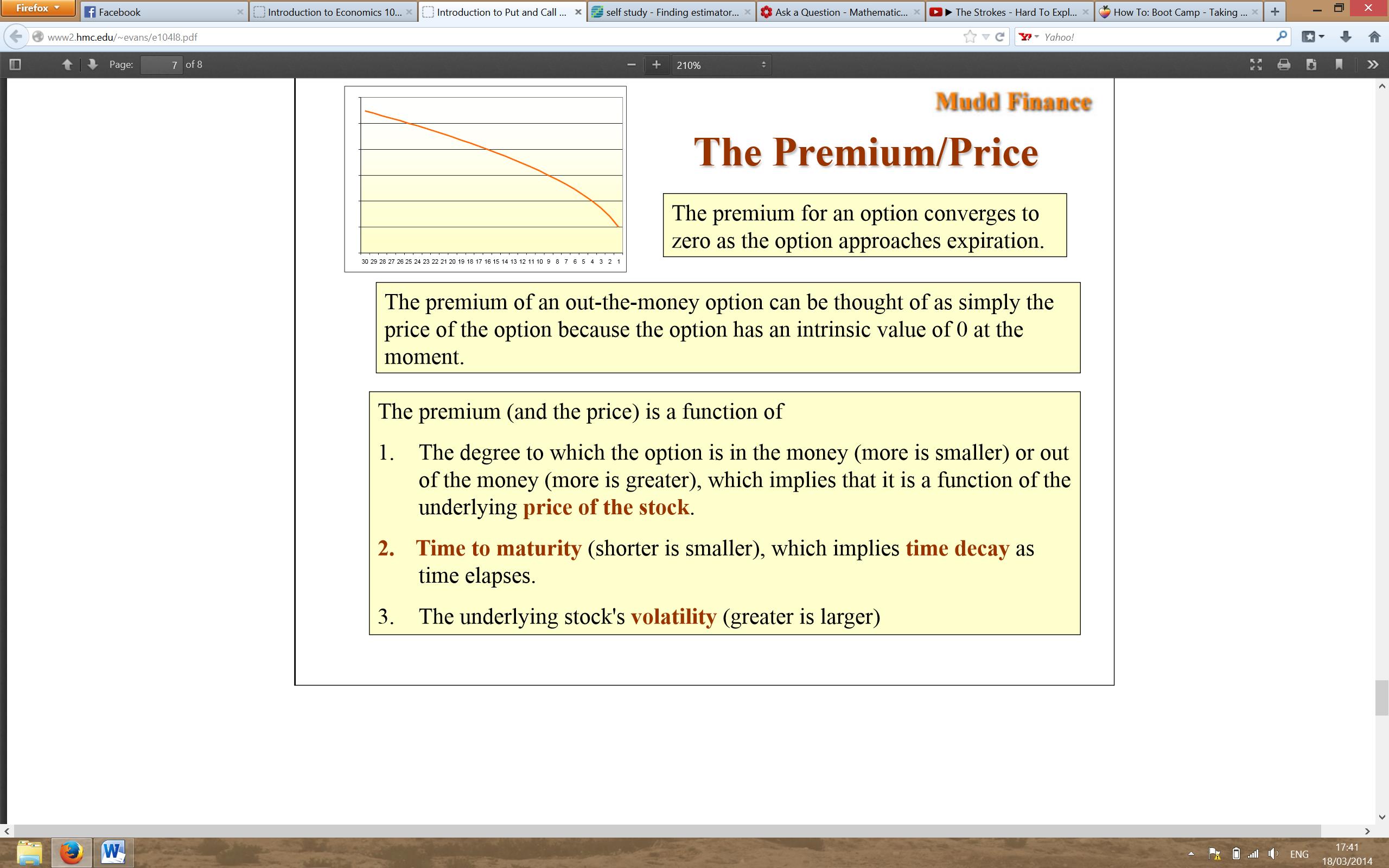
Time value is the value of an option beyond its intrinsic value and represents the potential for the option to gain additional value before expiration. It accounts for factors such as the time remaining until expiration, market volatility, and the expected price movement of the underlying asset. Time value decreases as the option approaches its expiration date. For options that are further away from expiration, time value tends to be higher, resulting in higher premium costs.
Volatility
Volatility refers to the degree of price fluctuation of the underlying asset. Higher volatility increases the potential for larger price swings, which in turn increases the likelihood of the option reaching a profitable state. Higher volatility generally leads to higher option premiums, as there is a greater probability of the option being worthy of exercise and capturing potential gains.
Interest Rates
Interest rates play a significant role in determining option premiums, especially for options that have a longer time to expiration. Higher interest rates increase the cost of carrying the underlying asset, which can influence the option’s premium. As interest rates rise, call options may have higher premiums, while put options may have lower premiums.
Dividends
For stocks that pay dividends, the timing and amount of dividend payments can impact option premiums. Generally, an impending dividend payment can decrease the premium of a call option and increase the premium of a put option. This adjustment accounts for the potential loss of dividend income for the buyer of the stock.
The Effects of Supply and Demand on Option Premiums
Supply and demand dynamics in the options market can affect option premiums as well. If there is a high demand for a particular option, its premium may increase due to increased competition among buyers. On the other hand, if there is a surplus of options contracts available, the premium may decrease. Market conditions, investor sentiment, and the overall trading activity in specific options contracts can drive changes in supply and demand, leading to fluctuations in premiums.
By understanding and analyzing these factors, traders and investors can better evaluate option premiums and make informed decisions in their options trading strategies. It’s important to consider these factors in conjunction with your market outlook, risk tolerance, and investment goals to optimize your options trading approach.
Intrinsic Value
Intrinsic value is a critical component in determining the price of an option and represents the amount of real value contained within the option. It is defined as the difference between the current price of the underlying asset and the strike price of the option. Depending on this difference, an option is classified as either in-the-money, at-the-money, or out-of-the-money.
In-the-Money (ITM)
A call option is considered in-the-money when the current price of the underlying asset is higher than the strike price. In this scenario, exercising the option would result in an immediate profit. For example, if the stock ABC is trading at $50 per share and you own a call option with a strike price of $45, your option has an intrinsic value of $5 ($50 – $45). The intrinsic value represents the profit that could be obtained by exercising the option and immediately selling the shares at the higher market price.
Similarly, a put option is in-the-money when the current price of the underlying asset is lower than the strike price. In this case, exercising the put option would allow you to sell the asset at a higher price than its current market value and generate a profit. For instance, if the stock XYZ is trading at $60 per share and you hold a put option with a strike price of $65, your option has an intrinsic value of $5 ($65 – $60).
At-the-Money (ATM)
An option is classified as at-the-money when the current price of the underlying asset is roughly equal to the strike price. In this situation, the option has no intrinsic value, as exercising it would not result in an immediate profit. For instance, if the stock PQR is trading at $40 per share and you possess a call option with a strike price of $40, the option is considered at-the-money.
Out-of-the-Money (OTM)
An option is out-of-the-money when the current price of the underlying asset is not favorable for exercise. In this case, exercising the option would lead to a loss, as it would be more beneficial to buy or sell the asset in the open market. For example, if the stock LMN is trading at $30 per share and you have a call option with a strike price of $35, your option is out-of-the-money, as there is no profit in exercising it.
The intrinsic value of an option sets a floor price for the option premium. In-the-money options have intrinsic value and will always have a higher premium than at-the-money or out-of-the-money options, which have no intrinsic value. It’s important to note that the premium of an option consists not only of intrinsic value but also time value, which represents the potential for the option to gain additional value before expiration.
Understanding the concept of intrinsic value is crucial in evaluating the potential profitability of an options contract. By analyzing the current price of the underlying asset relative to the strike price, traders and investors can make more informed decisions regarding the buying, selling, or exercising of options.
Time Value
Time value is a crucial component of option premiums and represents the additional value attributed to an option beyond its intrinsic value. It accounts for the potential for the option to gain value before its expiration date through changes in the underlying asset’s price, market conditions, and other factors.
Time value is influenced by several key factors:
Time Remaining Until Expiration
As time passes, the value of an option’s time value diminishes. This is because the longer an option has until expiration, the greater the likelihood that the underlying asset’s price may move in a favorable direction for the option holder. The closer an option gets to its expiration date, the less time there is for the asset’s price to change, leading to a decrease in its time value.
Market Volatility
Volatility is a measure of the price fluctuations in the underlying asset. Higher volatility increases the likelihood of large price swings, which can significantly impact the value of an option. When market volatility is high, options have a greater chance of moving into profitable territory, leading to higher time values. Conversely, when volatility is low, options may have lower time values, as the likelihood of significant price movements decreases.
Expected Price Movement
The expected price movement of the underlying asset also affects the time value of an option. If there is a high expectation for the asset to experience significant price changes, the option’s time value will be higher. This is because there is a greater likelihood of the option moving into a profitable state, and investors are willing to pay a higher premium for the potential gains.
Interest Rates
Interest rates play a role in determining the time value of an option, particularly for options with longer expiration dates. Higher interest rates increase the cost of holding the underlying asset, which can erode the option holder’s potential profits. As a result, options with longer expiration dates may have higher time values to account for the increased cost of carrying the position.
It’s important to note that time value is a perishable asset. As time passes, it gradually decays and approaches zero as the option approaches its expiration date. Traders and investors who buy options need to be aware of the time decay effect and carefully consider their timing and strategy to maximize their potential for profit.
Time value is an essential consideration when assessing the attractiveness and pricing of options contracts. By analyzing the time remaining until expiration, market volatility, expected price movement, and interest rates, traders and investors can better understand the potential for an option’s time value to contribute to its overall premium.
Volatility
Volatility is a crucial factor that influences the pricing of options and plays a significant role in determining their premiums. It refers to the degree of price fluctuation of the underlying asset and is a measure of the potential for large price swings. When it comes to options, higher volatility generally leads to higher premiums, while lower volatility tends to result in lower premiums.
There are two main types of volatility that impact option pricing:
Historical Volatility
Historical volatility measures the magnitude of past price movements of the underlying asset. It provides an objective assessment of how volatile the asset has been over a certain period and allows investors to gauge the potential range of price movements in the future. When historical volatility is high, it suggests that the asset has experienced significant price fluctuations, leading to higher option premiums.
Implied Volatility
Implied volatility reflects market expectations of future volatility and is derived from the current option prices. It takes into account various factors such as upcoming events, economic data releases, and market sentiment. Implied volatility is a key input in option pricing models, and its level directly impacts the premium of an option. When investors anticipate higher volatility in the future, implied volatility increases, resulting in higher option premiums.
Why is volatility important to option pricing? The rationale lies in the increased potential for large price movements. Higher volatility implies a greater likelihood of the underlying asset reaching a price level where an option may become profitable. Therefore, options on assets with higher volatility tend to have higher premiums due to the increased probability of generating a profit.
It’s important to note that volatility differs across various financial instruments and sectors. For example, technology stocks might have higher volatility compared to utility stocks due to their growth potential and market dynamics. Traders and investors need to consider the volatility of the underlying asset when evaluating options to ensure they align with their risk tolerance and investment objectives.
Additionally, understanding volatility can help traders employ specific options strategies. For example, in a high-volatility environment, options strategies like straddles or strangles may be more appealing as they benefit from larger price swings and provide opportunities for potential profits.
In summary, volatility plays a significant role in option pricing. Higher volatility increases the likelihood of large price movements, and as a result, leads to higher option premiums. It’s essential for traders and investors to monitor and assess the volatility of the underlying asset to make informed decisions when trading options and managing risk.
Interest Rates
Interest rates play a crucial role in the pricing of options and can significantly impact their premiums. When considering options, it’s important to understand how interest rates affect their value and why they are a key factor in the pricing equation.
The relationship between interest rates and option premiums can be explained through the concept of cost of carry. The cost of carry refers to the cost of holding the underlying asset required to support an options position.
Effect on Call Options
When interest rates rise, the cost of carrying the underlying asset increases. This increase in the cost of carry also affects call options. As interest rates go up, call options may have higher premiums to account for the increased cost of holding the underlying asset until expiration. Higher premiums ensure that the option writer is compensated for the higher cost of carrying the position.
Effect on Put Options
On the other hand, put options have an inverse relationship with interest rates. When interest rates rise, the cost of carrying the underlying asset also increases. As a result, the premium for put options may decrease. This decrease is due to the fact that the higher cost of carrying the underlying asset reduces the potential profit for put option holders, resulting in lower premiums.
It’s important to note that interest rates’ impact on option premiums is more pronounced for options with longer time to expiration. The longer the time remaining until expiration, the more significant the effect of interest rates on the option premiums.
Moreover, interest rates can also have an indirect impact on option premiums through their influence on the overall market dynamics. Changes in interest rates can affect investor sentiment, overall market volatility, and the demand for options. These factors can contribute to fluctuations in option premiums.
Traders and investors need to consider the prevailing interest rate environment when pricing and trading options. Monitoring changes in interest rates and their potential impact on option premiums can help in making informed decisions and managing risk effectively.
It’s important to keep in mind that interest rates are just one of many factors that affect option pricing. Other factors such as the underlying asset’s price, volatility, time remaining until expiration, and supply and demand in the options market also play significant roles.
In summary, interest rates have an impact on the pricing of options. Rising interest rates can lead to higher premiums for call options and potentially lower premiums for put options due to the increased cost of carrying the underlying asset. Understanding the relationship between interest rates and option premiums is essential for traders and investors to make informed decisions when trading options and managing their portfolios.
Dividends
Dividends are an important consideration when it comes to pricing options, particularly for stocks that pay dividends. Dividends are periodic cash payments made by companies to their shareholders as a way to distribute profits. The timing and amount of dividends can have an impact on option premiums.
For call options, dividends can decrease the premium, while for put options, dividends can increase the premium. Let’s explore how dividends affect option pricing in more detail:
Call Options
When a company announces a dividend payment, the stock price typically decreases by the dividend amount. This decrease in the stock price directly impacts the intrinsic value of call options. As the stock price decreases, the call option becomes less in-the-money or even out-of-the-money. As a result, the premium for call options may decrease to reflect the decreased likelihood of the option being exercised and capturing potential gains from the stock’s price appreciation. Therefore, call options generally have lower premiums when dividends are expected or paid.
Put Options
For put options, the impact of dividends is reversed. When a company pays a dividend, the stock price usually drops by the dividend amount. This decrease in the stock price can increase the value of a put option because it enhances the put option holder’s ability to sell the stock at a higher price. As a result, put options may have higher premiums to account for the increased potential profit from selling the stock at a higher price. Therefore, put options generally have higher premiums when dividends are expected or paid.
It’s important to note that the impact of dividends on option premiums may vary depending on the dividend amount, timing, and the strike price of the option relative to the stock price. Traders and investors need to consider these factors and evaluate the potential impact of dividends when making options trading decisions.
Furthermore, options pricing models, such as the Black-Scholes model, account for dividends by adjusting certain inputs. These adjustments help in accurately pricing options that are affected by dividend payments.
In summary, dividends can affect the pricing of options. Call options generally have lower premiums when dividends are expected or paid, as the stock price decreases. In contrast, put options may have higher premiums when dividends are expected or paid, as the stock price drops. Traders and investors should stay informed about dividend announcements and consider their potential impact on option premiums when analyzing and trading options.
The Effects of Supply and Demand on Option Premiums
Supply and demand dynamics play a significant role in determining the prices of options in the market. The interaction between buyers and sellers, driven by their perceived value and market outlook, influences the level of option premiums. Understanding the effects of supply and demand on option premiums is crucial for traders and investors.
When demand for a particular option outweighs the available supply, option premiums tend to increase. This occurs because buyers are willing to pay a higher price to secure the option contract, outbidding other potential buyers. The increased competition among buyers pushes the premium higher.
Conversely, when there is an excess supply of options contracts in the market compared to demand, premiums may decrease. With more sellers looking to offload their options contracts, they may have to lower their asking prices to attract buyers. This oversupply of options puts downward pressure on premiums.
Several factors can impact the supply and demand dynamics and consequently affect option premiums:
Market Sentiment
Optimistic or bullish market sentiment can drive up demand for call options, as investors seek to profit from potential price appreciation in the underlying asset. This increased demand for call options can lead to higher premiums. Conversely, in a bearish market environment, demand for put options may rise, driving up their premiums.
Implied Volatility
Changes in implied volatility, which reflects market expectations of future price swings, can impact supply and demand for options. Higher implied volatility often increases demand for options, as traders anticipate larger potential price movements and seek to hedge their positions or speculate on price changes. The increased demand can lead to higher premiums. Conversely, when implied volatility is low, demand for options may decrease, resulting in lower premiums.
Underlying Asset’s Price and Market Conditions
The price of the underlying asset and prevailing market conditions also influence supply and demand for options. When the price of the underlying asset increases or market conditions are favorable, demand for call options may rise, potentially driving up premiums. Conversely, when the price of the underlying asset decreases or market conditions are unfavorable, demand for put options may increase, affecting their premiums.
Supply and demand dynamics in the options market are constantly changing as new information becomes available and market participants adjust their strategies and positions. Monitoring these dynamics and understanding their impact on option premiums allows traders and investors to make informed decisions and potentially capitalize on pricing inefficiencies.
It’s important to note that supply and demand can also be impacted by institutional factors, such as options market makers or large institutions engaging in options strategies to hedge their positions. These factors can introduce additional complexities to the supply and demand dynamics of options and influence option premiums.
Overall, understanding the effects of supply and demand on option premiums provides valuable insights for traders and investors. By analyzing market sentiment, implied volatility, and the underlying asset’s price, they can better navigate the options market and identify potential opportunities.
Methods of Calculating Option Premiums
Option premiums are calculated using several mathematical models that take into account various factors such as the current price of the underlying asset, strike price, time to expiration, volatility, interest rates, and dividends. These models provide a framework for determining the fair value of an option and play a vital role in options pricing and trading strategies. Let’s explore some of the common methods used to calculate option premiums:
Black-Scholes Model
The Black-Scholes model is one of the most widely used methods for pricing options. Developed by economists Fischer Black and Myron Scholes in 1973, it provides an equation to estimate the theoretical value of European-style options. The Black-Scholes model takes into account factors such as the current stock price, strike price, time to expiration, volatility, interest rates, and dividends. By inputting these variables into the model, traders and investors can calculate the fair value of an option.
Binomial Model
The binomial model is another popular method for option pricing. Unlike the Black-Scholes model, the binomial model allows for the valuation of both European and American-style options. The model uses a tree-like structure to simulate possible price movements of the underlying asset over time. By using probabilities to model the likelihood of price movements, the binomial model calculates option values at each node within the tree, ultimately providing an estimate of the option’s fair value.
Other Approaches to Option Pricing
In addition to the Black-Scholes and binomial models, there are alternative methods for option pricing that take into account different assumptions and market conditions. These approaches include the Cox-Ross-Rubinstein (CRR) model, the Heston model, and the Monte Carlo simulation method. Each model has its own strengths and limitations and may be preferred in certain situations, such as when pricing options with complex features or when considering market conditions that deviate from the assumptions of the Black-Scholes model.
It’s important to note that option pricing models are theoretical in nature and provide estimates of option values based on certain assumptions. Market prices of options may deviate from these theoretical values due to various factors such as market supply and demand dynamics, liquidity, and market participant behavior.
Traders and investors often compare the calculated fair value of an option with its market price to identify potential opportunities for trading. If the market price is significantly different from the estimated fair value, there may be opportunities to buy undervalued options or sell overvalued options.
When using these pricing models, it’s essential to input accurate and up-to-date information for the underlying asset’s price, volatility, interest rates, and dividends to obtain more reliable estimates. Moreover, understanding the limitations and assumptions of each model is important for making informed decisions and managing risk effectively when trading options.
By utilizing these methods of calculating option premiums, traders and investors can better analyze options and make informed decisions based on a more accurate assessment of their fair value.
Black-Scholes Model
The Black-Scholes model is a widely used mathematical model for pricing options, particularly European-style options. Developed by economists Fischer Black and Myron Scholes in 1973, the model provides a framework for estimating the fair value of options based on several key variables.
The main assumptions behind the Black-Scholes model are:
- The underlying asset follows a geometric Brownian motion, meaning its price movements are continuous and random.
- The market is efficient, with no opportunities for risk-free arbitrage.
- There are no transaction costs or restrictions on short-selling.
- There are no dividends paid during the option’s time to expiration.
- Interest rates and market volatility are constant over the option’s lifespan.
Based on these assumptions, the Black-Scholes model provides a mathematical equation to calculate the theoretical value of European-style options. The model takes into account the current price of the underlying asset, the strike price of the option, the time remaining until expiration, the risk-free interest rate, and the volatility of the underlying asset.
The Black-Scholes equation calculates the value of a call option as:
C = S * N(d1) – X * e^(-rt) * N(d2)
Where:
- C represents the call option’s fair value
- S is the current price of the underlying asset
- N(d1) and N(d2) are the probabilities of the option expiring in-the-money based on the standard normal distribution
- X is the strike price of the option
- e is the mathematical constant approximately equal to 2.71828
- r is the risk-free interest rate
- t is the time remaining until expiration, expressed as a fraction of a year
The model also provides a formula for calculating the fair value of a put option, which is:
P = X * e^(-rt) * N(-d2) – S * N(-d1)
Where N(-d1) and N(-d2) represent the probabilities of the option expiring out-of-the-money.
The Black-Scholes model helps traders and investors estimate the fair value of options and compare it to their market prices. If the calculated fair value differs significantly from the market price, there may be opportunities to trade options that are overpriced or underpriced.
It’s important to note that the Black-Scholes model has its limitations and makes certain assumptions that may not always hold true in real-world market conditions. For example, it assumes constant volatility, which may not be the case in practice. Moreover, the model is most accurate with European-style options and may provide less accurate estimates for American-style options.
Despite its limitations, the Black-Scholes model remains a widely used and influential tool in options pricing. It has paved the way for further advancements in quantitative finance and continues to provide valuable insights into the fair valuation of options in financial markets.
Binomial Model
The binomial model is a popular mathematical method for pricing options, capable of valuing both European and American-style options. Unlike the Black-Scholes model, which assumes continuous price movements, the binomial model uses a discrete-time framework that considers a series of potential price movements in the underlying asset. It provides a tree-like structure to represent the possible paths that the underlying asset price can take over time.
The binomial model relies on several key factors:
- The current price of the underlying asset
- The strike price of the option
- The risk-free interest rate
- The time until expiration, divided into discrete periods
- The probability of an up movement and a down movement in the underlying asset’s price at each period
The model assumes that the price of the underlying asset can either go up or down by a certain percentage at each period. By using the probability of an up movement and a down movement, calculated based on the assumed volatility, the binomial model calculates the option’s fair value at each node within the tree.
Starting from the final period, the model works backward through the tree, calculating the option’s value at each node. At every node, the option’s value is the maximum between the intrinsic value (the difference between the current price of the underlying asset and the strike price) and the discounted expected value of the option at the next period.
By recursively calculating the option’s value at each node, the binomial model produces the fair value of the option at the initial node, representing the current price of the option. The model takes into account the impact of the underlying asset’s price movements, the time remaining until expiration, and the interest rate in determining the option’s price.
One of the advantages of the binomial model is its ability to price American-style options. These options can be exercised at any time before expiration, unlike European options that can only be exercised at expiration. The binomial model factors in the possibility of early exercise, allowing for a more accurate valuation of American-style options.
However, it’s important to note that while the binomial model can provide a more accurate estimate of fair value compared to the Black-Scholes model for options with complex features or early exercise possibilities, it can be computationally intensive for more elaborate option structures.
In summary, the binomial model offers a discrete-time framework for pricing options. By considering a series of possible price movements in the underlying asset and utilizing probabilities, it calculates option values at each node within a tree-like structure. The model is particularly useful for valuing American-style options and options with complex features. Traders and investors can incorporate the binomial model in their options pricing and trading strategies to obtain more accurate estimates of fair value.
Other Approaches to Option Pricing
In addition to the widely used Black-Scholes and binomial models, there are alternative methods for pricing options that take into account different assumptions and market conditions. These approaches provide alternative frameworks for estimating option premiums and can be useful in certain scenarios. Here are some other approaches to option pricing:
Cox-Ross-Rubinstein (CRR) Model
The Cox-Ross-Rubinstein (CRR) model is a variation of the binomial model that aims to improve the precision of option pricing. It introduces a modification to the probabilities used in the binomial model to ensure that the model replicates the continuous geometric Brownian motion assumption of the Black-Scholes model as the time periods become infinitesimally small. The CRR model provides more accurate pricing estimates for options and is widely used in practice.
Heston Model
The Heston model is a stochastic volatility model that can better capture the dynamics of asset price volatility compared to the constant volatility assumption of the Black-Scholes model. It introduces a process for modeling the volatility of the underlying asset that can change over time. The Heston model allows for more flexible and realistic pricing of options, particularly in markets with complex volatility patterns.
Monte Carlo Simulation
Monte Carlo simulation is a computational technique used to estimate option prices by simulating numerous possible price paths of the underlying asset. This approach randomly generates potential future prices using statistical methods and calculates the option’s value based on these simulated scenarios. By considering a large number of price paths, the Monte Carlo simulation provides a distribution of possible option values, allowing for a more comprehensive understanding of the option’s fair value and potential risks.
Other Variations and Custom Models
Besides the aforementioned models, there are various other variations and custom models that traders and researchers employ to suit specific needs. These models may incorporate different assumptions, such as jumps in asset prices or more complex stochastic processes for the underlying asset’s behavior. These custom models are often developed to account for specific market conditions or option features that may not align with the assumptions of traditional models.
It’s important to note that alternative option pricing models may require more computational resources and expertise to use effectively. Traders and investors should consider their specific requirements, market conditions, and assumptions when choosing an appropriate model for pricing options.
By utilizing alternative approaches to option pricing, traders and investors can gain a more nuanced perspective on option premiums. These models provide flexibility and accuracy in pricing options, allowing for better risk management and trading decisions in various market conditions.
Conclusion
Understanding how option premiums are calculated is essential for traders and investors in navigating the world of options trading. The factors influencing option premiums, such as intrinsic value, time value, volatility, interest rates, dividends, and supply and demand dynamics, all come into play when pricing these financial derivatives. By comprehending these factors, traders and investors can make more informed decisions about options positions, risk management, and trading strategies.
The Black-Scholes model and the binomial model are widely used methods for calculating option premiums, with each offering unique advantages. The Black-Scholes model is commonly employed for pricing European-style options and provides a formula that values options based on various inputs such as the underlying asset’s price, strike price, time to expiration, volatility, interest rates, and dividends. On the other hand, the binomial model accommodates both European and American-style options. It builds a tree-like structure to simulate potential price movements, enabling a more accurate pricing of options with complex features or early exercise possibilities.
Alternative approaches, including the Cox-Ross-Rubinstein (CRR) model, Heston model, and Monte Carlo simulation, offer additional flexibility and precision in option pricing by considering specific market conditions and features. These models cater to diverse needs and can aid traders and investors in effectively managing their options portfolios.
It’s important to keep in mind that option pricing models provide estimates of fair value based on certain assumptions, and market prices of options may deviate from these estimates due to factors like supply and demand dynamics. Market conditions, investor sentiment, and unforeseen events can impact option premiums beyond the mathematical calculations provided by these models.
In conclusion, comprehending the various factors affecting option premiums and utilizing appropriate pricing models empower traders and investors to make well-informed decisions when trading options. By assessing market conditions, considering risk tolerance, and conducting thorough analysis, individuals can optimize their options trading strategies and potentially enhance their financial outcomes in this dynamic and exciting financial market.
What's Hot
Latest Articles
Related Post

By: • Finance


By: • Finance

By: • Finance
By: • Finance
By: • Finance

By: • Finance


By: • Finance
By: • Finance

By: • Finance

By: • Finance