Home>Finance>How To Apply Accounting Number Format In Excel 2013

Finance
How To Apply Accounting Number Format In Excel 2013
Published: October 12, 2023
Learn how to apply the Accounting Number Format in Excel 2013 and streamline your finance tasks. Enhance your financial reporting with this simple tutorial.
(Many of the links in this article redirect to a specific reviewed product. Your purchase of these products through affiliate links helps to generate commission for LiveWell, at no extra cost. Learn more)
Table of Contents
- Introduction
- Step 1: Opening Excel 2013
- Step 2: Selecting the Cells to Format
- Step 3: Accessing the Format Cells Dialog Box
- Step 4: Choosing the Accounting Number Format
- Step 5: Adjusting Currency Symbol and Decimal Places
- Step 6: Applying the Accounting Number Format to Negative Numbers
- Step 7: Applying the Accounting Number Format to Dates and Times
- Step 8: Applying the Accounting Number Format to Fractions
- Conclusion
Introduction
Accounting Number Format is a popular formatting option in Excel 2013 that allows users to apply a consistent and professional look to numerical data. Whether you are a student, a business professional, or simply someone who needs to work with financial data, understanding how to apply the Accounting Number Format can greatly enhance your Excel skills and improve the presentation of your financial information.
The Accounting Number Format in Excel 2013 is designed to mimic the format used in financial reports. It is particularly useful for displaying monetary values, such as revenue, expenses, and balances, as it aligns decimal points and currency symbols for easier interpretation. By applying this format, you can create clear and organized spreadsheets that are visually appealing and easy to understand.
In this article, we will guide you through the steps of applying the Accounting Number Format in Excel 2013. We will explain how to select the cells you wish to format and access the Format Cells dialog box. We will also show you how to choose the Accounting Number Format, adjust currency symbols and decimal places, and apply the format to negative numbers, dates and times, and fractions.
By following this comprehensive tutorial, you will gain a solid understanding of how to use the Accounting Number Format to effectively present financial data in Excel 2013. Whether you are preparing financial statements, analyzing data for business purposes, or working on personal finance projects, the Accounting Number Format will help you create professional-looking spreadsheets that are both visually appealing and accurate.
Step 1: Opening Excel 2013
Before you can begin applying the Accounting Number Format in Excel 2013, you need to ensure that you have the software installed on your computer. If you do not have Excel 2013 installed, you can download it from the official Microsoft website or purchase a copy from a trusted retailer. Once you have Excel 2013 ready to go, follow these steps to open the software:
- Click on the “Start” button located at the bottom left corner of your computer screen.
- In the search bar, type “Excel 2013” or simply “Excel” and press Enter.
- The Excel 2013 application will appear in the search results. Click on it to launch the software.
- Alternatively, if you have a shortcut icon for Excel 2013 on your desktop, you can double-click on it to open the software.
- Once Excel 2013 is open, you will be greeted with a blank workbook, ready for you to start working on your spreadsheet.
Opening Excel 2013 allows you to access all the features and functionalities of the program, including the tools needed to apply the Accounting Number Format. It is important to ensure that you have the correct version of Excel installed, as the steps and options may vary slightly between different versions. If you are not using Excel 2013, you can still apply the Accounting Number Format in other versions, but the steps may be slightly different.
Now that you have successfully opened Excel 2013, you’re ready to move on to the next step of applying the Accounting Number Format: selecting the cells to format.
Step 2: Selecting the Cells to Format
Once you have Excel 2013 open and ready to go, the next step in applying the Accounting Number Format is to select the cells that you want to format. This step is crucial as it determines which cells will have the Accounting Number Format applied to them. Follow these steps to select the desired cells:
- Click and drag your mouse over the cells that you want to format. You can select a single cell, multiple cells, or even an entire range of cells by clicking and dragging from the starting cell to the ending cell.
- If the cells you want to format are spread across different areas of your worksheet, hold down the “Ctrl” key on your keyboard and click on each cell individually to select them.
- If you want to select an entire column or row, simply click on the column or row header to highlight it.
- To select the entire worksheet, click on the “Select All” button located at the intersection of the row and column headers, or use the keyboard shortcut “Ctrl + A”.
By selecting the cells that you want to format, you ensure that the Accounting Number Format will only be applied to the desired range of cells, rather than the entire worksheet. This allows you to have more control and flexibility over how your data is displayed.
It’s important to note that you can apply the Accounting Number Format to cells that already contain data, as well as to blank cells that you plan to fill in later. Additionally, you can modify the selection of cells at any time before applying the format by simply clicking and dragging to include or exclude cells as needed.
Now that you have selected the cells to format, you’re ready to move on to the next step: accessing the Format Cells dialog box.
Step 3: Accessing the Format Cells Dialog Box
Once you have selected the cells that you want to format in Excel 2013, the next step is to access the Format Cells dialog box. This dialog box contains various formatting options, including the Accounting Number Format. Here’s how you can access it:
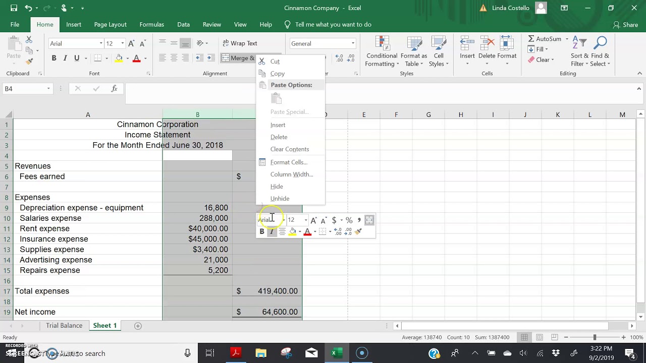
- Right-click on the selected cells. A context menu will appear with various options.
- From the context menu, select the “Format Cells” option. Alternatively, you can access the Format Cells dialog box by going to the “Home” tab on the Excel ribbon, clicking on the “Format” button in the “Cells” group, and selecting “Format Cells” from the drop-down menu.
- The Format Cells dialog box will open, displaying several tabs that represent different formatting categories, such as Number, Alignment, Font, and Border.
- Switch to the “Number” tab if it’s not already selected. The Number tab contains various number formats that you can apply to your selected cells, including the Accounting Number Format.
Accessing the Format Cells dialog box provides you with a wide range of options to customize the formatting of your cells. In addition to the Accounting Number Format, you can also explore other formatting options available in the dialog box, such as currency symbols, decimal places, date and time formats, and more.
By having access to the Format Cells dialog box, you have the flexibility to adjust the formatting based on your specific needs. Whether you are working with financial data, scientific figures, or general numerical values, the Format Cells dialog box allows you to choose the appropriate format and presentation style to make your data easily understandable and visually pleasing.
Now that you have accessed the Format Cells dialog box, you are ready to proceed to the next step: choosing the Accounting Number Format.
Step 4: Choosing the Accounting Number Format
After accessing the Format Cells dialog box in Excel 2013, the next step is to choose the Accounting Number Format. This format is specifically designed for financial data and provides a professional and consistent look to monetary values. Follow these steps to apply the Accounting Number Format to your selected cells:
- In the Format Cells dialog box, make sure the “Number” tab is selected. This tab contains various number formats that you can apply to your cells.
- In the “Category” section, scroll down or click on “Accounting” to select it. This will change the available options in the “Type” section below.
- Review the options in the “Type” section and choose the desired format. The options include different variations of the Accounting Number Format, such as with or without currency symbols, different decimal places, and even negative number formatting.
- As you select different formats, you can preview the changes in the “Sample” section of the Format Cells dialog box. This allows you to see how the format will appear before applying it to your cells.
- Once you have chosen the desired Accounting Number Format, click the “OK” button at the bottom of the Format Cells dialog box. The selected cells will now be formatted accordingly.
By choosing the Accounting Number Format, you ensure that your monetary values are displayed consistently, with aligned decimal places and appropriate currency symbols. This format is particularly useful when working with financial statements, budgeting, or any other scenario that involves monetary data.
It’s important to note that you can always go back to the Format Cells dialog box if you want to make changes to the Accounting Number Format or apply a different format altogether. Simply repeat Step 3 to access the dialog box and make the necessary adjustments.
Now that you have chosen the Accounting Number Format for your selected cells, you can proceed to the next step: adjusting currency symbols and decimal places if needed.
Step 5: Adjusting Currency Symbol and Decimal Places
After choosing the Accounting Number Format for your selected cells in Excel 2013, you have the option to adjust the currency symbol and decimal places to further customize the presentation of your financial data. Follow these steps to make these adjustments:
- Select the cells that have the Accounting Number Format applied to them.
- Right-click on the selected cells and choose “Format Cells” from the context menu. Alternatively, go to the “Home” tab on the Excel ribbon, click on the “Format” button in the “Cells” group, and select “Format Cells” from the drop-down menu.
- In the Format Cells dialog box, navigate to the “Number” tab if it’s not already selected.
- Ensure that the “Accounting” category is selected, and in the “Type” section, you will see a sample preview of the format applied to the selected cells.
- To adjust the currency symbol, click on the “Symbol” dropdown menu next to the “Type” section. Choose the desired currency symbol or select “None” if you don’t want to display any currency symbol.
- To adjust the decimal places, look for the “Decimal places” dropdown menu in the “Type” section. Select the desired number of decimal places or choose “Automatic” for Excel to determine the appropriate decimal places based on the data.
- As you make changes to the currency symbol and decimal places, you can preview the adjustments in the “Sample” section of the Format Cells dialog box.
- Once you are satisfied with the adjustments, click the “OK” button to apply the changes to the selected cells.
By adjusting the currency symbol and decimal places, you can tailor the Accounting Number Format to match your specific financial data and presentation preferences. This level of customization ensures that your monetary values are accurately formatted and visually appealing.
It’s worth mentioning that you can revisit the Format Cells dialog box at any time to make further adjustments or modify the formatting settings. Simply follow Step 3 to access the dialog box and make the necessary changes.
Now that you have learned how to adjust the currency symbol and decimal places, you can proceed to the next step: applying the Accounting Number Format to negative numbers.
Step 6: Applying the Accounting Number Format to Negative Numbers
When working with financial data in Excel 2013, it’s important to properly format negative numbers to ensure clarity and accuracy. Fortunately, the Accounting Number Format allows you to easily apply formatting to negative numbers. Follow these steps to apply the Accounting Number Format to negative numbers:
- Select the cells that contain negative numbers and have the Accounting Number Format applied to them.
- Right-click on the selected cells and choose “Format Cells” from the context menu. Alternatively, go to the “Home” tab on the Excel ribbon, click on the “Format” button in the “Cells” group, and select “Format Cells” from the drop-down menu.
- In the Format Cells dialog box, navigate to the “Number” tab if it’s not already selected.
- Ensure that the “Accounting” category is selected, and in the “Type” section, you will see a sample preview of the format applied to the selected cells.
- Below the “Type” section, you will find the “Negative numbers” area. This section allows you to choose how negative numbers are displayed.
- By default, Excel displays negative numbers using parentheses. If you prefer a different formatting style, such as using a minus sign (-) or displaying negative numbers in red, you can select the desired option from the dropdown menu.
- To customize the appearance of negative numbers further, click on the “Format” button next to the dropdown menu. This will open the Format Cells dialog box, where you can choose different formatting options such as font color, boldness, and more.
- Once you have made the necessary adjustments to the negative number formatting, click the “OK” button to apply the changes to the selected cells.
By applying the Accounting Number Format to negative numbers, you can clearly distinguish them from positive numbers and ensure that the financial data is correctly interpreted.
Remember, you can always go back to the Format Cells dialog box and modify the formatting settings for negative numbers at any time. Simply follow Step 3 to access the dialog box and make the desired changes.
Now that you have learned how to apply the Accounting Number Format to negative numbers, you can proceed to the next step: applying the format to dates and times.
Step 7: Applying the Accounting Number Format to Dates and Times
Excel 2013 allows you to apply the Accounting Number Format not only to numerical data but also to dates and times. This can be helpful when working with financial records that include transaction dates or durations. Follow these steps to apply the Accounting Number Format to dates and times:
- Select the cells that contain dates or times and have the Accounting Number Format applied to them.
- Right-click on the selected cells and choose “Format Cells” from the context menu. Alternatively, go to the “Home” tab on the Excel ribbon, click on the “Format” button in the “Cells” group, and select “Format Cells” from the drop-down menu.
- In the Format Cells dialog box, navigate to the “Number” tab if it’s not already selected.
- Ensure that the “Accounting” category is selected, and in the “Type” section, you will see a sample preview of the format applied to the selected cells.
- Excel automatically detects date and time values and applies the appropriate format based on your system settings. However, if you prefer a specific date or time format, you can choose the desired option from the “Type” dropdown menu.
- If you want to customize the date or time format further, click on the “Format” button next to the “Type” dropdown menu. This will open the Format Cells dialog box, where you can select from various date and time formatting options.
- Once you have made the necessary adjustments to the date or time formatting, click the “OK” button to apply the changes to the selected cells.
By applying the Accounting Number Format to dates and times, you can ensure that they are displayed consistently and aligned with the rest of your financial data. This can be particularly useful when working with financial reports that include date-based analysis or time durations.
Remember, you can revisit the Format Cells dialog box and modify the date or time formatting settings at any time. Simply follow Step 3 to access the dialog box and make the desired changes.
Now that you have learned how to apply the Accounting Number Format to dates and times, you can proceed to the final step: applying the format to fractions.
Step 8: Applying the Accounting Number Format to Fractions
Excel 2013 offers the flexibility to apply the Accounting Number Format to fractions, allowing you to present fractional values in a consistent and professional manner. Whether you are working with financial calculations or need to display fractional data, follow these steps to apply the Accounting Number Format to fractions:
- Select the cells that contain fraction values and have the Accounting Number Format applied to them.
- Right-click on the selected cells and choose “Format Cells” from the context menu. Alternatively, go to the “Home” tab on the Excel ribbon, click on the “Format” button in the “Cells” group, and select “Format Cells” from the drop-down menu.
- In the Format Cells dialog box, navigate to the “Number” tab if it’s not already selected.
- Ensure that the “Accounting” category is selected, and in the “Type” section, you will see a sample preview of the format applied to the selected cells.
- By default, Excel uses the Accounting Number Format to display fractions where the denominator is less than 100. If you have fractions with a larger denominator, you will need to choose a different fraction format.
- To customize the fraction format, click on the “Symbol” dropdown menu next to the “Type” section. Select “Fraction” from the list of options.
- Next to the “Fraction” option, you will find a “Type” dropdown menu that allows you to select different fraction formats, such as “Up to one digit” or “Up to two digits”. Choose the desired format that matches your data.
- As you make changes to the fraction formatting, you can preview the adjustments in the “Sample” section of the Format Cells dialog box.
- Once you are satisfied with the fraction format, click the “OK” button to apply the changes to the selected cells.
By applying the Accounting Number Format to fractions, you can clearly present fractional values and ensure consistency in your financial data. Whether you are working with invoices, measurements, or any other scenario that involves fractions, this format will help you maintain a professional and organized appearance.
Remember, you can always revisit the Format Cells dialog box and modify the fraction formatting settings as needed. Simply follow Step 3 to access the dialog box and make the desired changes.
Congratulations! You have now learned how to apply the Accounting Number Format to fractions in Excel 2013. By following these steps, you can effectively format your financial data and create visually appealing spreadsheets.
Conclusion
Mastering the application of the Accounting Number Format in Excel 2013 is an essential skill for anyone working with financial data. With this formatting option, you can present numerical, date, time, and fraction values in a consistent and professional manner. By following the step-by-step guide outlined in this article, you can easily apply the Accounting Number Format and tailor it to meet your specific needs.
Throughout the tutorial, we covered the process of opening Excel 2013 and selecting the cells to format. We then explored how to access the Format Cells dialog box and choose the Accounting Number Format from the number category. Additionally, we discussed how to adjust currency symbols, decimal places, and customize the formatting of negative numbers, dates and times, as well as fractions.
Applying the Accounting Number Format not only enhances the visual appeal of your spreadsheets but also ensures that financial data is presented accurately and professionally. Whether you are creating financial reports, analyzing budgeting data, or managing personal finances, this formatting option will make your data easier to interpret and comprehend.
Remember to consider the specific requirements of your financial data and adjust the formatting accordingly. Pay attention to the placement of currency symbols, the number of decimal places, and the appropriate way to display negative numbers, dates, times, and fractions, depending on your specific use case.
By mastering the Accounting Number Format in Excel 2013, you will be equipped with the skills to create visually appealing and informative spreadsheets that effectively communicate financial data and analysis.
So, give it a try and start applying the Accounting Number Format in Excel 2013 to enhance your financial presentations and make your data shine!
What's Hot
Latest Articles
Related Post

By: • Finance
By: • Finance
By: • Finance
By: • Finance
By: • Finance

By: • Finance

By: • Finance

By: • Finance

By: • Finance

By: • Finance

By: Sunny • Finance


By: • Finance