
Finance
How To Use Accounting Number Format In Excel
Published: October 10, 2023
Learn how to use the accounting number format in Excel for effective financial management and analysis. Improve your finance skills with this easy-to-follow guide.
(Many of the links in this article redirect to a specific reviewed product. Your purchase of these products through affiliate links helps to generate commission for LiveWell, at no extra cost. Learn more)
Table of Contents
- Introduction
- How to apply the Accounting Number Format in Excel
- Step 1: Select the cells you want to format
- Step 2: Go to the Home tab
- Step 3: Find the Number group
- Step 4: Click on the drop-down menu next to the Number Format box
- Step 5: Select the Accounting option
- Step 6: Customize the format if desired
- Step 7: Apply the format to the selected cells
- Conclusion
Introduction
When it comes to managing financial data in Excel, accuracy and clarity are vital. The accounting number format in Excel is a powerful tool that allows you to display numbers in a professional and easy-to-read format, similar to what you would see in a financial statement or balance sheet.
By using the accounting number format, you can align decimal points, add dollar signs or currency symbols, and apply thousand separators to your numbers. This format helps to enhance readability and ensure consistency in your financial calculations, making it easier for you and other users to understand and interpret the data.
In this article, we will guide you through the steps to apply the accounting number format in Excel, so you can present your financial data with precision and professionalism. Whether you are a small business owner, an accountant, or simply someone who wants to enhance the appearance of your Excel worksheets, this guide will help you leverage the accounting number format to its fullest potential.
How to apply the Accounting Number Format in Excel
Applying the accounting number format in Excel is a straightforward process that can be accomplished in just a few simple steps. Here’s a step-by-step guide:
- Select the cells you want to format: Begin by selecting the cells in your Excel worksheet that you want to apply the accounting number format to. You can click and drag to select a range of cells or hold down the Ctrl key while clicking to select individual cells.
- Go to the Home tab: Once you’ve selected the desired cells, navigate to the Home tab in the Excel ribbon. This tab is typically located at the top of the screen and includes various formatting options.
- Find the Number group: Within the Home tab, locate the Number group. This group contains different number formatting options that you can apply to your selected cells.
- Click on the drop-down menu next to the Number Format box: In the Number group, you’ll notice a box that displays the current formatting of the selected cells. Click on the drop-down arrow next to this box to reveal a list of formatting options.
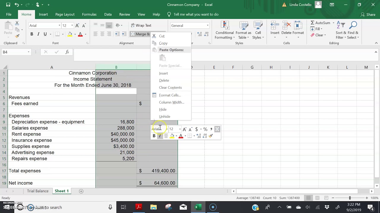
- Select the Accounting option: From the drop-down menu, scroll through the list of formatting options and select “Accounting”. This option is specifically designed to format numbers in a professional accounting style, with currency symbols, decimal alignment, and thousand separators.
- Customize the format if desired: If you wish to customize the accounting number format further, you can click on the “More Number Formats” option at the bottom of the drop-down menu. This will open a dialog box with additional formatting options, such as choosing a specific currency symbol or adjusting decimal places.
- Apply the format to the selected cells: Once you are satisfied with the formatting options, click on the “OK” button to apply the accounting number format to the selected cells. Excel will instantly display the numbers in the chosen format, making them easier to read and understand.
By following these steps, you can quickly and efficiently apply the accounting number format to your Excel worksheets. This format not only enhances the visual appeal of your financial data but also ensures accuracy and consistency in your calculations. Whether you’re preparing a budget, analyzing sales figures, or presenting financial reports, the accounting number format in Excel is a valuable tool to showcase your data professionally.
Step 1: Select the cells you want to format
The first step in applying the accounting number format in Excel is to select the cells that you want to format. This allows you to specify which cells will display the formatted numbers. Follow these simple instructions to select the desired cells:
- Click and drag to select a range of cells: If you want to format a continuous range of cells, you can click and drag your mouse across the cells. This action will highlight and select all the cells within the dragged area.
- Hold down the Ctrl key and click to select individual cells: If you want to format specific cells that are not in a continuous range, you can hold down the Ctrl key on your keyboard and click on each desired cell. This action allows you to select multiple individual cells.
- Select an entire column or row: To apply the accounting number format to an entire column or row, simply click on the column letter or row number. This action will select all the cells within that column or row.
By selecting the cells that you want to format, you have control over which numbers will be displayed in the accounting number format. This step is crucial for ensuring that you apply the formatting only where necessary, avoiding any unintended changes to your Excel worksheet.
Step 2: Go to the Home tab
Once you have selected the cells that you want to format, the next step is to navigate to the Home tab in Excel. The Home tab is where you’ll find a wide range of formatting options, including the accounting number format. Follow these steps to access the Home tab:
- Open your Excel worksheet: Launch Microsoft Excel on your computer and open the worksheet that contains the cells you want to format.
- Locate the Home tab: The Home tab is typically located at the top of the Excel window. It is one of the primary tabs in the Excel ribbon, along with other tabs such as Insert, Page Layout, and Formulas.
- Select the Home tab: Click on the Home tab to activate it. Once selected, the Home tab will display various formatting options that you can use to customize your Excel worksheet.
The Home tab in Excel is a central hub for formatting and manipulating data. It provides quick access to essential tools and features that can help you organize and present your information effectively. By navigating to the Home tab, you’re ready to proceed to the next step of applying the accounting number format to your selected cells.
Step 3: Find the Number group
Once you have opened your Excel worksheet and selected the Home tab, the next step is to locate the Number group. The Number group is where you’ll find various number formatting options, including the accounting number format. Here’s how you can find the Number group in Excel:
- Look for the “Number” or “Number Format” group: Scan the Home tab for a group that specifically relates to number formatting. In most versions of Excel, this group is labeled as either “Number” or “Number Format”. It is usually located towards the center or right-hand side of the Home tab.
- Identify the Number group icons: The Number group typically consists of several icons or buttons that represent different number formatting options. These icons may include symbols like dollar signs, percentage signs, and decimal point alignment indicators.
- Note additional formatting options: Within the Number group, you may also find other number formatting options, such as date formats, time formats, and scientific notation. These options may be housed in separate sections or displayed as dropdown menus.
Locating the Number group is essential as it serves as the entry point to access the accounting number format and other number formatting options in Excel. Once you have identified the Number group, you are now ready to proceed to the next step of applying the accounting number format to your selected cells.
Step 4: Click on the drop-down menu next to the Number Format box
After you have found the Number group in the Home tab, the next step is to click on the drop-down menu next to the Number Format box. This menu contains a list of formatting options that can be applied to your selected cells. Follow these instructions to access the drop-down menu:
- Locate the Number Format box: Within the Number group, you will see a box that displays the current number formatting of the selected cells. The box may show the “General” format by default.
- Click on the drop-down arrow: To reveal the list of available number formatting options, click on the small arrow icon or downward-facing triangle next to the Number Format box. This action will open the drop-down menu.
The drop-down menu provides a wide range of number formatting choices, such as currency formats, percentage formats, and date formats. It allows you to select the specific formatting style you want to apply to your selected cells.
By clicking on the drop-down menu next to the Number Format box, you have now accessed the list of number formatting options available in Excel. The next step is to choose the accounting number format to apply to your selected cells.
Step 5: Select the Accounting option
Once you have opened the drop-down menu next to the Number Format box in the Excel Home tab, the next step is to select the Accounting option. The Accounting option is specifically designed to format numbers in a professional accounting style, complete with currency symbols, decimal alignment, and thousand separators. Follow these steps to choose the Accounting format:
- Scroll through the formatting options: Within the drop-down menu, scroll through the list of available number formatting options. You will see a range of choices, including General, Number, Currency, Percentage, and more.
- Locate the Accounting option: As you scroll through the list, look for the Accounting option. It is often represented by a dollar sign ($) and is labeled as “Accounting” or “Accounting Number Format”.
- Select the Accounting option: Once you have found the Accounting option, click on it to select it. This action will apply the accounting number format to your selected cells.
By selecting the Accounting option, you ensure that your numbers are displayed in a professional accounting format, which is commonly used in financial statements, reports, and balance sheets. The format includes features like currency symbols, decimal alignment, and thousand separators, making your data more visually appealing and easier to read.
After selecting the Accounting option, you are now ready to proceed to the next step, where you can further customize the accounting number format if desired.
Step 6: Customize the format if desired
After selecting the Accounting option for your selected cells, you have the option to further customize the format to suit your preferences. Excel provides additional options to personalize the accounting number format, such as choosing a specific currency symbol or adjusting the number of decimal places. Follow these steps to customize the format:
- Click on “More Number Formats”: At the bottom of the drop-down menu, you will see an option called “More Number Formats”. Click on this option to open a dialog box with advanced formatting options.
- Explore the formatting options: In the “Format Cells” dialog box, you’ll find a wide range of formatting options to customize the accounting number format. You can choose different currency symbols, adjust decimal places, add or remove thousand separators, and more.
- Preview the changes: As you make changes to the format, you will see a live preview of how the numbers in your selected cells will appear. This allows you to visualize the impact of your formatting choices before applying them.
- Save your custom format: If you have customized the accounting number format and want to use it again in the future, you can save it as a custom format. Simply click on the “Custom” category in the “Format Cells” dialog box and click on the “Add” button to save your custom format for future use.
Customizing the accounting number format gives you the flexibility to adjust it according to your specific needs and preferences. Whether you want to use a different currency symbol or modify the decimal places, Excel provides the tools to tailor the format to your requirements.
Once you have customized the accounting number format to your satisfaction, you can proceed to the final step of applying the format to your selected cells.
Step 7: Apply the format to the selected cells
After selecting the accounting number format and customizing it according to your preferences, the final step is to apply the format to your selected cells. By doing so, you will see the numbers in your cells instantly transformed into the accounting number format. Follow these instructions to apply the format:
- Click on the “OK” button: In the “Format Cells” dialog box, once you have finished customizing the accounting number format, click on the “OK” button. This will close the dialog box and save your formatting changes.
- Observe the transformed numbers: After applying the format, the numbers in your selected cells will now be displayed in the accounting number format. You will see currency symbols, aligned decimal points, and thousand separators, making the data more visually appealing and easier to read.
- Review and make adjustments if necessary: Take a moment to review the formatted numbers in your cells. If you notice any inconsistencies or if the formatting does not meet your expectations, you can go back to the Home tab, open the Number Format box, and make additional adjustments as needed.
By applying the accounting number format to your selected cells, you have successfully transformed your data into a professional and easily understandable format. This format is particularly useful for financial calculations, reports, and any other instances where accuracy and clarity are essential.
Remember, you can always modify or remove the accounting number format by selecting the cells again, accessing the Number Format box, and choosing a different format or selecting the General format to remove any specific formatting.
With the accounting number format successfully applied to your selected cells, you can present your financial data with confidence and professionalism.
Conclusion
The accounting number format in Excel is a powerful tool that allows you to present financial data in a professional and visually appealing format. By following the step-by-step guide outlined in this article, you can easily apply the accounting number format to your selected cells, enhancing readability and improving the accuracy of your financial calculations.
Through the selection of the desired cells, navigation to the Home tab, and selection of the Number group, you can access the accounting number format options. By clicking on the drop-down menu next to the Number Format box, you can choose the Accounting option and instantly transform your numbers into a format commonly used in financial statements and reports.
Furthermore, Excel provides the flexibility to further customize the accounting number format. By clicking on “More Number Formats,” you can adjust settings such as currency symbols, decimal places, and thousand separators to meet your specific requirements. With a live preview of the changes, you can ensure that the formatting aligns perfectly with your intended presentation style.
Once you are satisfied with the customized format, applying it to the selected cells is a simple matter of clicking “OK” in the Format Cells dialog box. The numbers in your cells will be instantly transformed into the accounting number format, showcasing your financial data with professionalism and accuracy.
Remember, you can always revisit the formatting options and make adjustments as needed. Excel provides the flexibility to modify or remove the accounting number format easily, allowing you to adapt to changing requirements or preferences.
In conclusion, by leveraging the accounting number format in Excel, you can enhance the presentation of financial data, accurately convey information, and facilitate better comprehension of your worksheets. Mastering this tool will help you create visually appealing and professional-looking spreadsheets that impress your colleagues, clients, and stakeholders.
What's Hot
Latest Articles
Related Post
By: • Finance

By: • Finance

By: • Finance

By: • Finance

By: • Finance

By: • Finance

By: • Finance
By: • Finance
By: • Finance

By: • Finance

By: • Finance

By: • Finance

By: • Finance

By: • Finance