How To Make A Cash Flow Diagram In Excel

(Many of the links in this article redirect to a specific reviewed product. Your purchase of these products through affiliate links helps to generate commission for LiveWell, at no extra cost. Learn more)

Introduction

Welcome to the world of finance! Whether you are a business owner, an investor, or simply interested in managing your personal finances, having a clear understanding of your cash flow is essential. A cash flow diagram is a powerful tool that visually represents the inflows and outflows of cash over a given period of time. By creating a cash flow diagram in Excel, you can gain valuable insights into the timing and magnitude of your cash flows.

In this article, we will guide you through the process of creating a cash flow diagram in Excel. We will break down each step and provide you with practical tips to ensure your diagram is accurate and informative. Whether you are a beginner or an Excel pro, this article will equip you with the necessary knowledge to create an effective cash flow diagram.

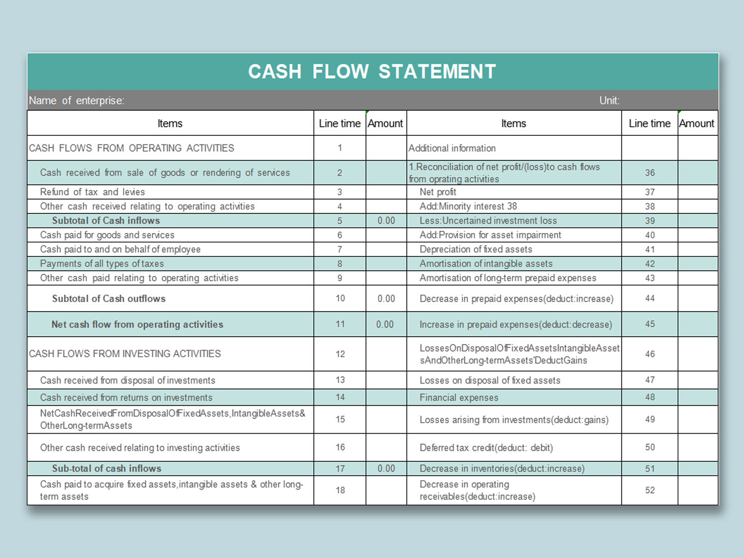
But before we dive into the details, let’s briefly discuss what a cash flow diagram represents. A cash flow diagram illustrates the movement of cash in and out of a business or personal account. It helps you visualize the timing and amount of cash inflows and outflows, allowing you to assess the overall financial health of your endeavors.

Having a clear understanding of your cash flow can aid in making informed decisions about budgeting, investment opportunities, and managing financial risks. By creating a cash flow diagram, you can easily identify periods of cash surplus or deficit, analyze trends and patterns, and spot potential areas for improvement.

Now that we understand the importance of a cash flow diagram, it’s time to roll up our sleeves and get started with creating one in Excel. So let’s move on to the first step: opening Excel and setting up the worksheet.

Step 1: Opening Excel

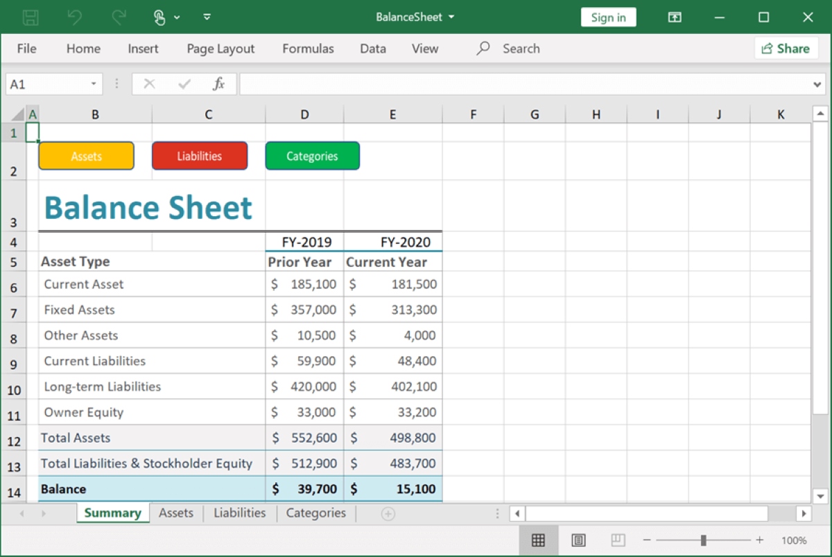
The first step in creating a cash flow diagram in Excel is to open the software. Excel is a widely used spreadsheet program that offers a range of features and tools for financial analysis and modeling. If you don’t have Excel installed on your computer, you can download a free trial version or use an alternative spreadsheet program.

Once you have opened Excel, you will be greeted with a blank workbook. This is where you will be creating your cash flow diagram. The workbook consists of multiple worksheets, with each worksheet representing a separate tab at the bottom of the screen. For our cash flow diagram, we will be working on a single worksheet.

To create a new worksheet, simply click on the “+ ” button located at the bottom-left corner of the screen. This will open a new blank worksheet where you can begin setting up your cash flow diagram.

Alternatively, you can use the keyboard shortcut Ctrl + N to open a new workbook. This will automatically open a new blank worksheet where you can start working on your cash flow diagram.

Once you have opened a new worksheet, you’re ready to move on to the next step: creating the header for your cash flow diagram. The header will serve as a title for your diagram and provide key information about the time period and the currency used.

Before we proceed, it’s worth mentioning that Excel offers a wide range of formatting options, such as fonts, colors, and borders, to customize the appearance of your cash flow diagram. Don’t be afraid to experiment with different formatting styles to make your diagram visually appealing and easy to interpret.

With Excel opened and a new worksheet created, let’s continue to step 2 where we will learn how to create the header for our cash flow diagram.

Step 2: Creating the Header

Now that you have opened Excel and created a new worksheet for your cash flow diagram, it’s time to add a header to your worksheet. The header will provide essential information about the time period and currency used in your cash flow diagram.

To create the header, begin by selecting the top row of your worksheet. You can do this by clicking and dragging the mouse across the entire row or by clicking on the row number at the left side of the screen. Once the row is selected, you can format it by changing the font, font size, and alignment.

The header should include key details such as the name of your cash flow diagram, the time period it covers, and the currency used. For instance, you can enter “Cash Flow Diagram” in cell A1 to serve as the main title. In the adjacent cells, you can enter the time period (e.g., “Month”, “Year”) and the currency symbol (e.g., “$”, “€”) respectively.

For consistency and clarity, it’s important to align the header text in a consistent manner. You can choose to center-align the main title in cell A1 and left-align the time period and currency symbols in the adjacent cells. This will make your header visually appealing and easy to read.

Additionally, you might want to consider formatting the header row with bold text or applying background color to make it stand out. You can do this by selecting the header row and using the formatting options available in the toolbar. Remember, the goal is to make your cash flow diagram visually appealing and easy to understand.

Once you have created the header, you can proceed to the next step of creating your cash flow diagram, which involves entering the time periods along the first column of your worksheet. This will allow you to track the cash flows over specific intervals, whether it’s months, quarters, or years.

With the header created, you are now ready to populate the worksheet with the necessary time periods. Continue reading to learn more about step 3: entering the time periods.

Step 3: Entering the Time Periods

In step 2, we created the header for our cash flow diagram, including the title, time period, and currency information. Now, in step 3, we will focus on entering the time periods along the first column of our worksheet.

Before we begin, it’s important to determine the appropriate time intervals for your cash flow diagram. This will depend on the nature of your financial analysis. For example, if you are tracking monthly cash flows, you will enter the months of the year (e.g., January, February, March) in the first column. If you prefer to track cash flows on a quarterly basis, you might enter the quarters (e.g., Q1, Q2, Q3) instead.

To enter the time periods, select the first column of your worksheet by clicking on the column letter at the top of the screen. Once the column is selected, you can begin entering the time periods in each cell. Start from the second row of the column (cell A2) to leave room for the header.

If you prefer to manually enter the time periods, you can simply type them into the corresponding cells. Alternatively, you can use Excel’s autofill feature to automatically populate the cells based on the pattern you provide.

For example, if you have entered “January” in cell A2, you can click and drag the bottom right corner of the cell (the fill handle) downwards to autofill the subsequent cells with the following months (e.g., February, March, April, and so on). Excel will recognize the pattern and fill in the cells accordingly.

If you are using quarters instead, you can enter “Q1” in cell A2 and use the autofill feature to populate the subsequent cells with “Q2”, “Q3”, and so on.

Remember, the purpose of entering the time periods is to create a framework for tracking your cash flows over specific intervals. Make sure the time periods align with your financial analysis objectives and accurately represent the time frame of your cash flow data.

With the time periods entered, we can move on to the next step: entering the cash inflows into our cash flow diagram. This step will allow us to capture the money coming into our account during the specified time intervals.

Continue reading to learn more about step 4: entering the cash inflows.

Step 4: Entering the Cash Inflows

Now that we have set up the header and entered the time periods in our cash flow diagram, we can move on to the next step: entering the cash inflows. Cash inflows represent the money that flows into your account during the specified time intervals.

To enter the cash inflows, start by selecting the first cell under the “Cash Inflows” column, which is usually the second column of your worksheet. By default, this will be cell B2 if you followed the previous steps.

Now, consider the specific sources of your cash inflows. This could include revenue from sales, client payments, rental income, or any other sources of income. Enter each individual cash inflow in the respective cells, aligning them with the corresponding time periods.

For example, if you are tracking monthly cash flows and your first source of cash inflow is from sales, enter the sales revenue for the month of January in cell B2. Continue entering the cash inflows for each month in the subsequent cells under the “Cash Inflows” column.

Remember to use appropriate formatting, such as using the currency format for the cash inflow values. You can do this by selecting the cells containing cash inflow values and using the formatting options available in Excel’s toolbar. This will present your data in a clear and readable format.

If you have multiple sources of cash inflows, you can create separate columns for each source. For example, you can have one column for sales revenue, another for client payments, and so on. This will provide a detailed breakdown of your cash inflows and allow for better analysis of where your money is coming from.

With the cash inflows entered, our cash flow diagram is starting to take shape. In the next step, we will move on to entering the cash outflows, which represent the expenses or payments that occur during the specified time intervals.

Keep reading to learn more about step 5: entering the cash outflows.

Step 5: Entering the Cash Outflows

After entering the cash inflows into our cash flow diagram, it’s time to focus on the next component: entering the cash outflows. Cash outflows represent the expenses or payments that occur during the specified time intervals.

To enter the cash outflows, select the first cell under the “Cash Outflows” column, which is typically the third column of your worksheet. By default, this will be cell C2 if you followed the previous steps.

Consider the different types of expenses or payments you need to account for in your cash flow diagram. This could include rent, utilities, salaries, loan repayments, inventory costs, or any other expenses incurred during the given time periods.

Enter each individual cash outflow in the respective cells, aligning with the corresponding time periods. For example, if you are tracking monthly cash flows and your rent expense for January is $1,000, enter that amount in cell C2. Continue entering the cash outflows for each month in the subsequent cells under the “Cash Outflows” column.

Similar to the cash inflows, use appropriate formatting, such as the currency format, for the cash outflow values. This will help to clearly represent your expenses in a readable format.

If you have multiple categories of cash outflows, you can create separate columns for each category just like you did for cash inflows. This allows for better categorization and analysis of your expenses. It also provides a comprehensive overview of where your money is going and helps in identifying areas for potential cost savings.

Remember, the accuracy and completeness of your cash outflow entries are crucial for an accurate representation of your financial situation. Take the time to review your expenses and ensure that all significant outflows are included in your cash flow diagram.

With the cash inflows and outflows entered, our cash flow diagram is nearly complete. In the next step, we will calculate the net cash flow, which shows the difference between the total cash inflows and outflows for each time period.

Continue reading to learn more about step 6: calculating the net cash flow.

Step 6: Calculating the Net Cash Flow

After entering the cash inflows and outflows in our cash flow diagram, it’s time to calculate the net cash flow for each time period. The net cash flow represents the difference between the total cash inflows and outflows, giving us an indication of whether we have a positive or negative cash flow.

To calculate the net cash flow, select the first cell under the “Net Cash Flow” column, which is typically the fourth column of your worksheet. By default, this will be cell D2 if you followed the previous steps.

In the first cell, you can use a simple formula to subtract the cash outflows (column C) from the cash inflows (column B). The formula will look something like “=B2 – C2”. This subtracts the recorded expenses from the recorded income, giving you the net cash flow for that specific time period.

After entering the formula in the first cell, you can use Excel’s autofill feature to copy the formula to the remaining cells in the “Net Cash Flow” column. Excel will automatically adjust the cells references based on the pattern of the formula.

If the net cash flow is positive, it means you have more cash inflows than outflows during that time period, indicating a surplus of cash. Conversely, if the net cash flow is negative, it means your outflows exceed your inflows, indicating a cash deficit.

Formatting the net cash flow column is optional, but you can choose to use conditional formatting to highlight positive cash flows in green and negative cash flows in red. This makes it easier to visually identify periods of cash surplus or deficit at a glance.

The net cash flow is a crucial metric in determining the overall financial performance and viability of your business or personal finances. By analyzing the net cash flow over time, you can gain insights into your cash management and make informed decisions to improve your financial standing.

With the net cash flow calculated, we are now ready to move on to the final step: creating the cash flow diagram itself. This visual representation will provide a clear and concise summary of your cash flow situation.

Continue reading to learn more about step 7: creating the cash flow diagram.

Step 7: Creating the Cash Flow Diagram

Now that we have entered the cash inflows, outflows, and calculated the net cash flow for each time period, it’s time to create the cash flow diagram. The cash flow diagram visually represents the movement of cash in and out of your account over the specified time intervals, providing a clear snapshot of your financial situation.

To create the cash flow diagram in Excel, we will use a combination of data visualization tools and formatting options. Here’s how:

1. Select the cells containing the time periods, cash inflows, outflows, and net cash flow data.
2. Click on the “Insert” tab in Excel’s toolbar and choose a suitable chart type for your cash flow diagram. Common chart types for cash flow diagrams include column charts or line charts.
3. Excel will generate a default chart based on the selected data. You can customize the appearance of the chart by right-clicking on various chart elements, such as the axes, labels, and legend, and selecting formatting options.
4. Add a chart title that clearly conveys the purpose of the diagram, such as “Cash Flow Analysis” or “Monthly Cash Flow.”
5. Consider adding data labels to the chart to provide numerical context for the cash inflows, outflows, and net cash flow values.
6. Format the chart to improve readability and visual appeal. This can include adjusting the font size, color schemes, and adding gridlines or other visual aids.
7. Lastly, consider adding a short description or key takeaways from the cash flow diagram in a separate text box, located near or below the chart. This summary can provide additional context and insights for the reader.

Remember, the purpose of the cash flow diagram is to provide a visual representation of your cash flow data, making it easier for you and others to interpret and understand your financial situation. Thus, it’s important to ensure the chart is clear, concise, and visually appealing.

Once you have created the cash flow diagram, take a moment to review and analyze the chart. Look for patterns, trends, and anomalies to gain a deeper understanding of your cash flow dynamics. This analysis can help you make strategic decisions to optimize your cash flow, improve profitability, and manage financial risks.

Congratulations! You have successfully created a cash flow diagram in Excel. By regularly updating and analyzing this diagram, you will gain valuable insights into your cash flow, enabling you to make informed financial decisions and achieve your financial goals.

With the cash flow diagram completed, we have reached the end of our step-by-step guide. We hope this article has provided you with the knowledge and confidence to create and utilize cash flow diagrams effectively. Remember to save your work and keep your cash flow diagram updated to reflect the most accurate and up-to-date financial information.

Thank you for reading, and happy cash flow management!

Conclusion

Understanding and managing your cash flow is crucial for financial success, whether you are a business owner or an individual looking to optimize your personal finances. Creating a cash flow diagram in Excel can provide you with a visual representation of your cash inflows and outflows, making it easier to track and analyze your financial situation.

In this article, we have covered step-by-step instructions for creating a cash flow diagram in Excel. Starting from opening Excel and setting up the worksheet, to entering the time periods, cash inflows, and cash outflows, and finally calculating the net cash flow and creating the cash flow diagram itself, you now have a comprehensive guide to follow.

By following these steps and customizing them according to your specific needs and financial goals, you can gain valuable insights into your cash flow, identify trends, and make informed decisions to improve your financial well-being.

Remember, a well-managed cash flow is vital for ensuring solvency, meeting financial obligations, and seizing opportunities for growth. Regularly updating and analyzing your cash flow diagram will help you stay on top of your finances, anticipate future cash needs, and make strategic financial decisions.

Don’t forget to take advantage of Excel’s formatting options and tools to enhance the visual appeal and readability of your cash flow diagram. A well-presented and visually appealing diagram can effectively communicate your financial situation to stakeholders, lenders, or potential investors.

In conclusion, mastering the art of creating cash flow diagrams in Excel is an essential skill for effective financial management. By harnessing the power of this tool, you can gain insights, make informed decisions, and ultimately achieve long-term financial success.

So grab your Excel spreadsheet, follow the steps outlined in this article, and start creating your own cash flow diagram today. Take control of your cash flow and unlock the potential for financial growth and stability.